tinygrad-notes
Shapetracker
examples were tested on commit a2a4ff30dcfafc8e7763303e9d8f0955900e8617 (in case things go out of date)
Suppose you have a 2 by 2 matrix containing values 1, 2, 3, 4. These four numbers are not stored in memory as a matrix, but as a linear strip. As such, you need a strategy to know that when you access the element at second row, first column, you are referring to the third element in the memory layout. That’s one of the motivations of shapetracker.
In this example, such a strategy can be illustrated as row_number * 2 + column_number equals the memory index (things
may be off by one depending on whether you count from zero or from one).
Here, the number 2 is called a stride. A stride refers to how many steps to take when you increment the value. Because going from the first element of one row, to the next row, involves skipping 2 elements, the stride for the row is 2. Similarly, the stride for the column (moving from one column to the next) is 1.
going from first row -->1 2
to the second row   --->3 4
skips two elements
You can see that in the equation above 1 is just omitted. Using row and column is not very scalable when you have larger dimensions. Hence, a general way to express this is by the dimension. Row is the 0th dimension, column is the 1st dimension. We can say that our zeroth dimension has a stride of 2, and first dimension has a stride of 1. These two values actually are the input to the shapetracker implementation:
View.create(shape=(2, 2), strides=(2, 1))
Here’s a tool for visualization: https://mesozoic-egg.github.io/shape-stride-visualizer/#/shape-stride
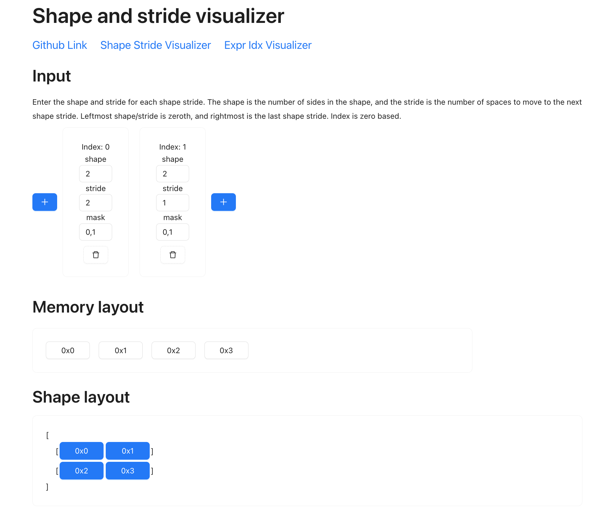
The top boxes refers to the dimensions you have. “Index 0” is dimension 0, “Index 1” is dimension 1. Within each dimension you put in the shape, stride, and mask. The memory layout now shows the four elements that are physically represented on the storage, and each has a memory address (0x00, 0x01, 0x02, 0x03). Then in the shape layout section, you can see how they are transformed into the shape that a shapetracker specifies, in this case, as a matrix. Note how each element maps to a certain position, for example, the element at 0x02 is the element on the second row, first column.
Note that a mask for a dimension refers to the start and end (inclusive) value that’s valid. The blue highlight refers to the values that are valid here. If you put the mask value for the zeroth dimension as “0, 0”, then only the first row will be highlighted.
This is a powerful concept, because we can now manipulate complex shape without changing the data. For example, if I want to transpose the matrix, so that instead of
[
  0x00, 0x01
  0x02, 0x03
]
I want:
[
  0x00, 0x02
  0x01, 0x03
]
You can easily achieve it by just flipping the strides:
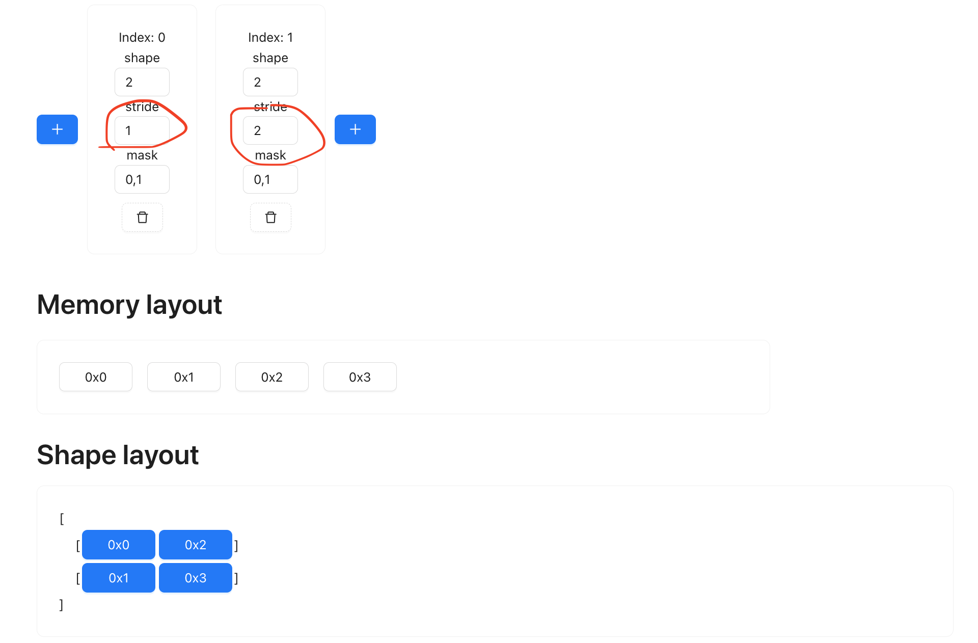
Note how the memory layout didn’t change? This is a nice thing to have, it means we are manipulating the tensor at almost zero cost. Sometimes you may transpose something, only to later transpose it back. If every transpose requires you to physically move the memory content, the computation will be slow. Doing it symbolically saves a lot of compute time.
There are a few layers of abstraction in the shapetracker API, let’s start from the bottom: View
from tinygrad.shape.view import View

# The two by two matrix is represneted as shape being (2, 2), strides being (2, 1)
a = View.create(shape=(2, 2), strides=(2, 1))

# In order to get the "strategy" we talked about (row * 2 + col), we call a special method:
idx, valid = a.to_indexed_uops()

# This method returns two objects. The first one is the access strategy I kept referring to, the second is for the mask.
# Let's focus on the first.
print(idx)

# If you print it, it may look a bit scary:
# UOp(Ops.ADD, dtypes.int, arg=None, src=(
#   UOp(Ops.ADD, dtypes.int, arg=None, src=(
#     x1:=UOp(Ops.CONST, dtypes.int, arg=0, src=()),
#     UOp(Ops.MUL, dtypes.int, arg=None, src=(
#       UOp(Ops.RANGE, dtypes.int, arg=0, src=(
#          x1,
#         UOp(Ops.CONST, dtypes.int, arg=3, src=()),)),
#       x5:=UOp(Ops.CONST, dtypes.int, arg=2, src=()),)),)),
#   UOp(Ops.MUL, dtypes.int, arg=None, src=(
#     UOp(Ops.RANGE, dtypes.int, arg=1, src=(
#        x1,
#        x5,)),
#     UOp(Ops.CONST, dtypes.int, arg=1, src=()),)),))
# Fortunately, there's a render method to show you something more sane:
print(idx.render())
# ((ridx0*2)+ridx1)
# This is the equivalent to "row * 2 + col"!
Keep in mind that .render() method is just for debugging, it’s the scary looking UOp AST that’s actually used to
render the access pattern when doing kernel computation. In fact, if you follow the AST tree, you should notice that
it actually translates to the readable render output:
The outer most node is an addition, this is the + sign. The first child is yet another addition, it adds a zero const, and a multiplication. We can deduce that the zero is some artifacts that’s not shown. THe multiplication multiplies two things: the first is a range, ranging from zero to three. This is the ridx0. the second is a const, value is 2.
The second child is a multiplication, between a range and 1. The range is ranging from zero to two which is ridx1.
Stride of zero
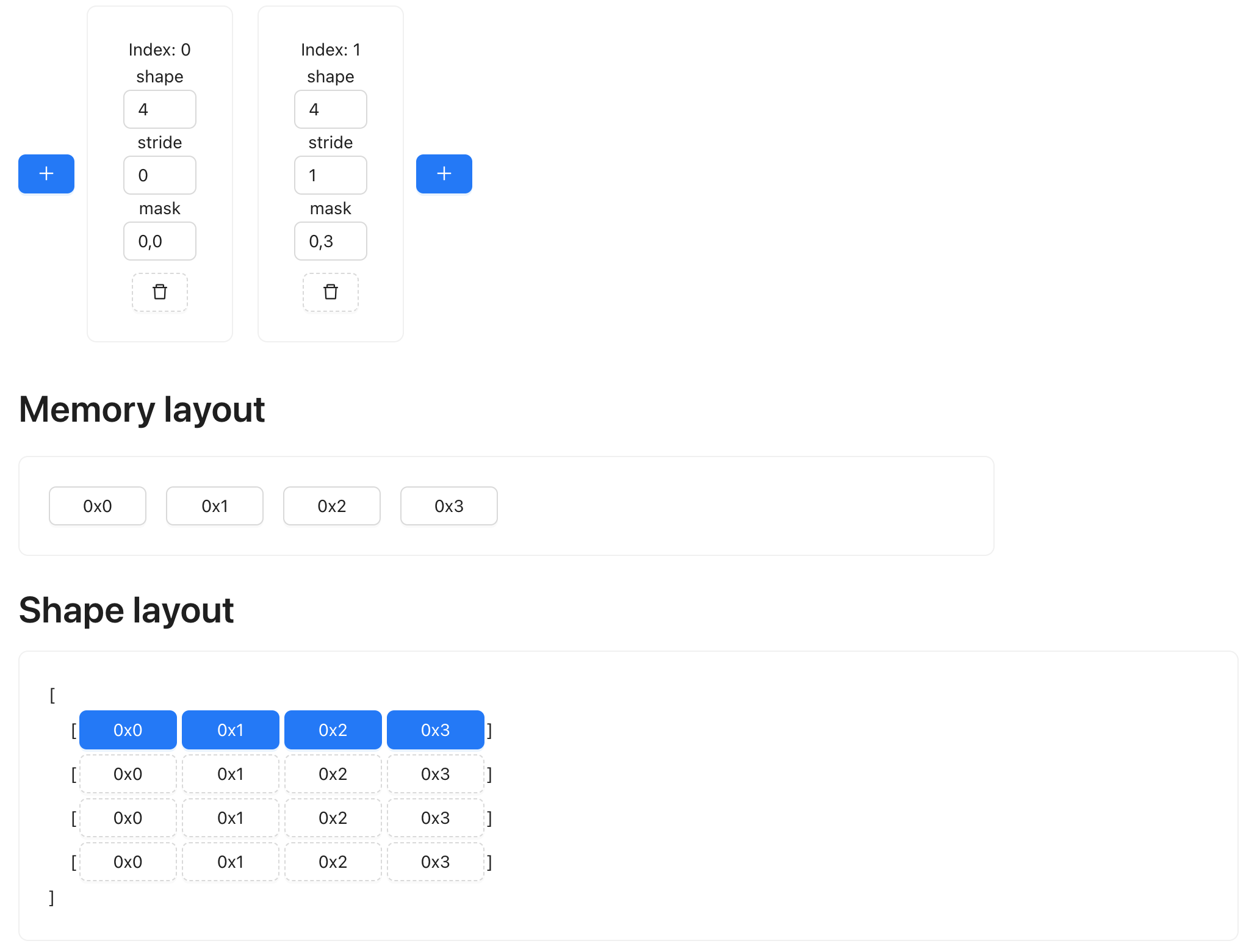
Having stride value being zero means you are taking the same element regardless of how many steps you take in that direction. For example, we may have a single row of data, and want to repeat it four times.

We can repeat in the row (0th) dimension. To expand it four times, we simply set the shape of dimension zero to value 4, and set its stride to 0:
Elements with gaps
Sometimes the memory layout is not contiguous, and there could be a gap between, say, the first and second row of data. This could happen because of slicing operation (for example, you might want just the even rows of a grid). Regardless of the use case, we can easily represent it with shapetracker too:
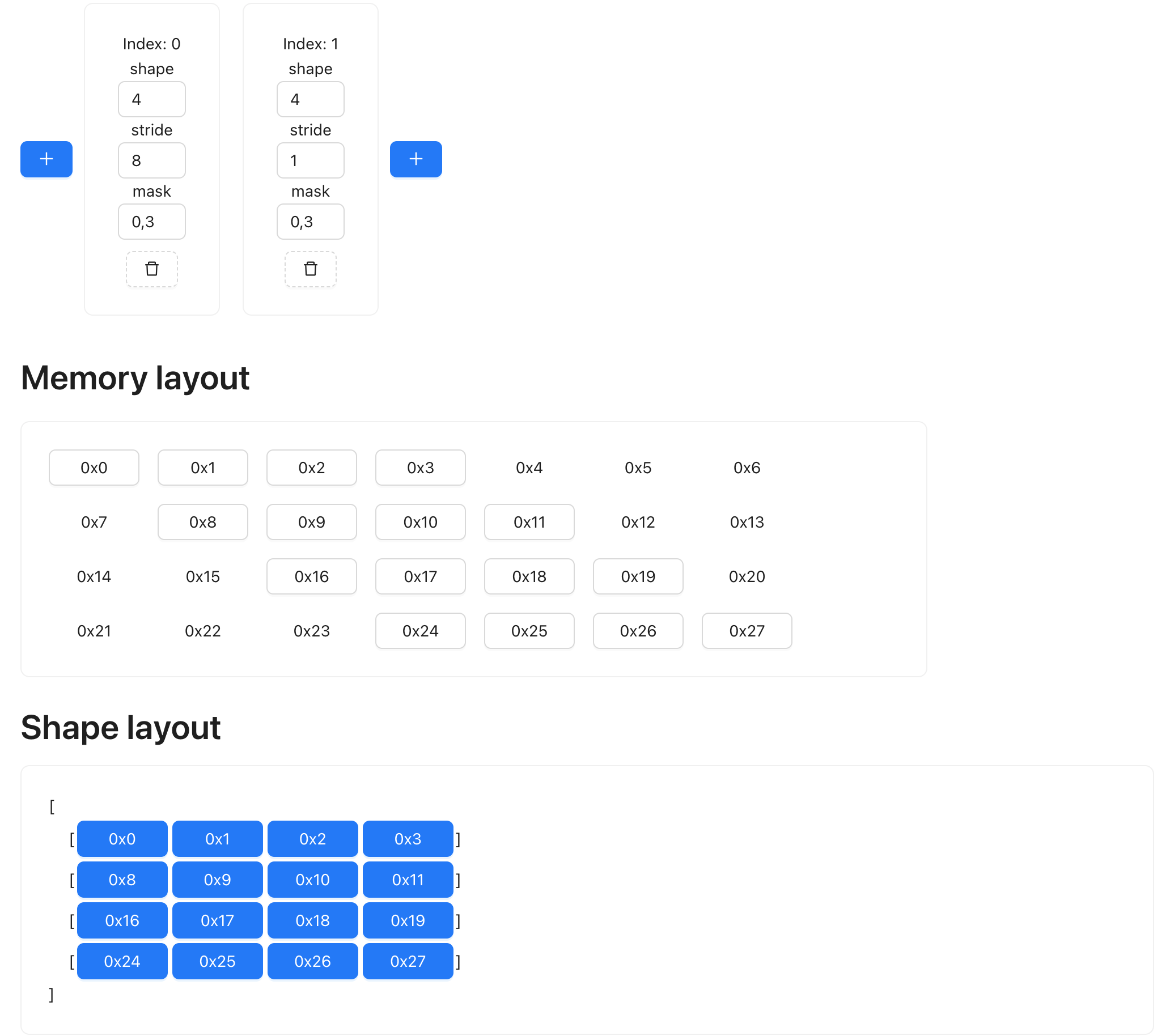
See how the memory layout has some gaps, and every row of the data is 4 elements apart?
Multi views
So far I have been dealing with shapes that can be represented with just 1 view. This means that given a shape, a stride, you can reconstruct the full tensor by indexing into the correct position in its linear memory data layout. This isn’t always the case with certain transformations though. Suppose we have a matrix of shape 3 by 2, then we transpose it, and then we reshape it back to 3 by 2, is there a way to represent it with a single pair of shape and stride?
 (3,2)                        (2,3)                    (3,2)
0x00 0x01   transpose    0x00 0x02 0x04  reshape     0x00 0x02
0x02 0x03 ------------>  0x01 0x03 0x05 ---------->  0x04 0x01
0x04 0x05                                            0x03 0x05
So despite the final result being still (3,2), the data is not the same before. We can look at how tinygrad handles such a situation:
a = View.create(shape=(3, 2), strides=(2,1))

# Transpose it
a = a.permute((1, 0))
print(a.shape) # (2, 3)
print(a.strides) # (1, 2)

a = a.reshape((3, 2))
print(a)
The returned value is actually None, because a single view cannot be reshaped to accommodate it. In other words, tinygrad detects that the desired layout cannot be represented with just a single pair of shape and stride. That brings us to the actual objects that is used for a general case, the Shapetracker class. You can think of it just as a container that can hold multiple views. Let’s rewrite our example:
from tinygrad.shape.shapetracker import ShapeTracker

a = ShapeTracker.from_shape((3, 2))
a = a.permute((1, 0))
a = a.reshape((3, 2))
print(a)
# ShapeTracker(views=(View(shape=(2, 3), strides=(1, 2), offset=0, mask=None, contiguous=False), View(shape=(3, 2), strides=(2, 1), offset=0, mask=None, contiguous=True)))
So we have two views now. Let’s get the index expression:
idx, valid = a.to_indexed_uops()
print(idx.render())
# (((((ridx0*2)+ridx1)%3)*2)+(((ridx0*2)+ridx1)//3))
It’s definitely a lot more complicated than the “row * 2 + col” example, but the visualizer has a mode to handle this too.
First we look at the variable, ridx0 refers to the 0th dim, which ranges from 0 to 2 (Recall that the shape is 3 by 2).
ridx1 refers to 1st dim, ranging from 0 to 1 (shape is 2). And we can compute all the combinations between the two variables
and find out what the layout should look like, on the expr viewer: https://mesozoic-egg.github.io/shape-stride-visualizer/#/expr-idx
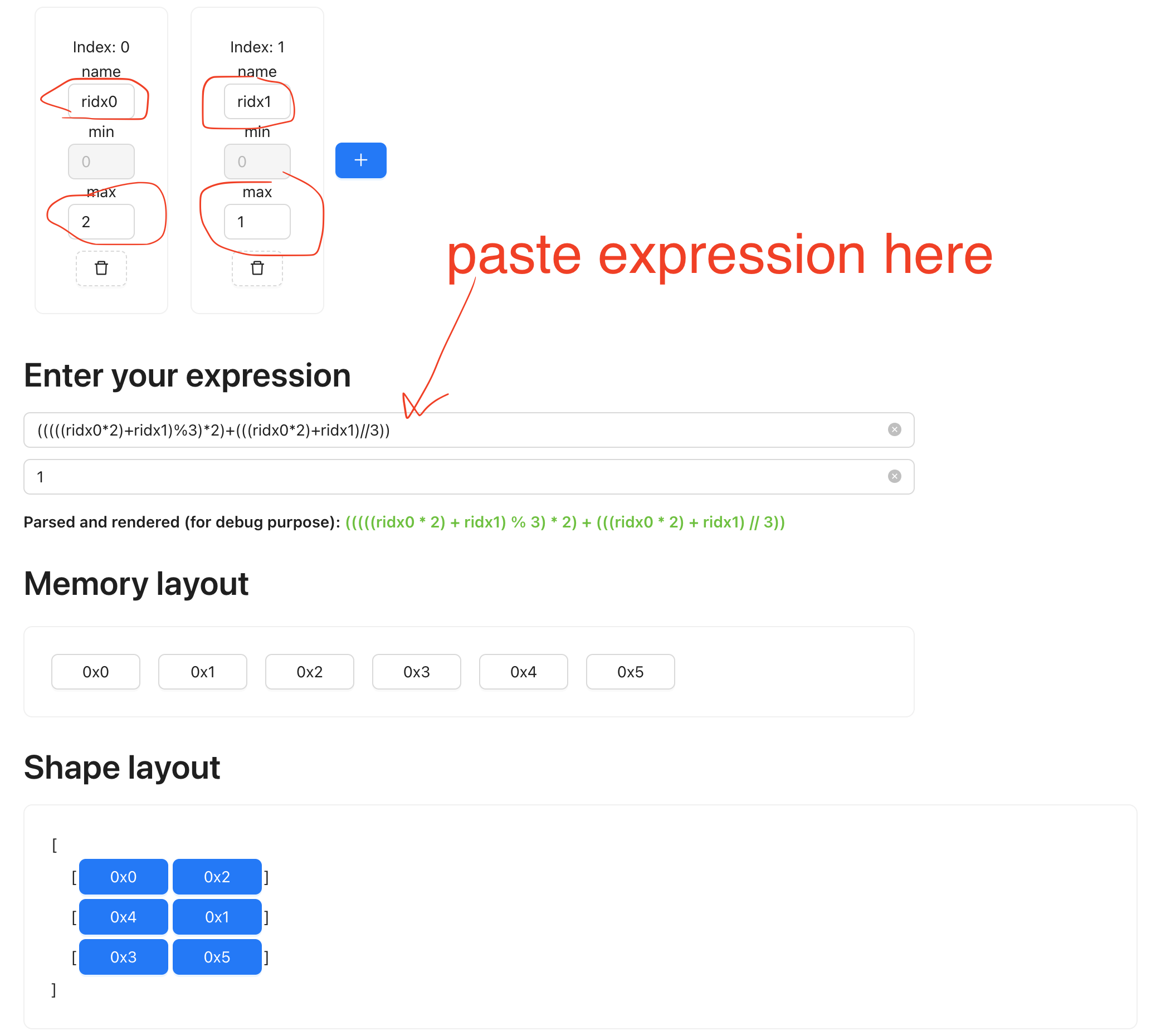
Make sure you put in the correct variable name, min and max value and paste in the expression. The second box is for the “valid”
variable, in our case, everything is valid because we didn’t apply any mask. Typing in a 1 means True for all.
You can see that the rendered output is what we have gotten when writing it out by hand.
Multiview implementation
How does multi views get rendered? Let’s peek at the implementation and break it down:
def views_to_indexed_uops(views: Tuple[View, ...], _idxs:Optional[Tuple[UOp, ...]]=None) -> Tuple[UOp, UOp]:
  idx, valid = views[-1].to_indexed_uops(_idxs)
  for view in reversed(views[0:-1]):
    view = view.minify()
    acc, idxs = 1, []
    for d in reversed(view.shape):
      idxs.append((idx//acc)%d)
      acc *= d
    idx, valid = view.to_indexed_uops(idxs[::-1], valid)
  return idx, valid
Recall what the two views look like:
View(shape=(2, 3), strides=(1, 2), offset=0, mask=None, contiguous=False)
View(shape=(3, 2), strides=(2, 1), offset=0, mask=None, contiguous=True))
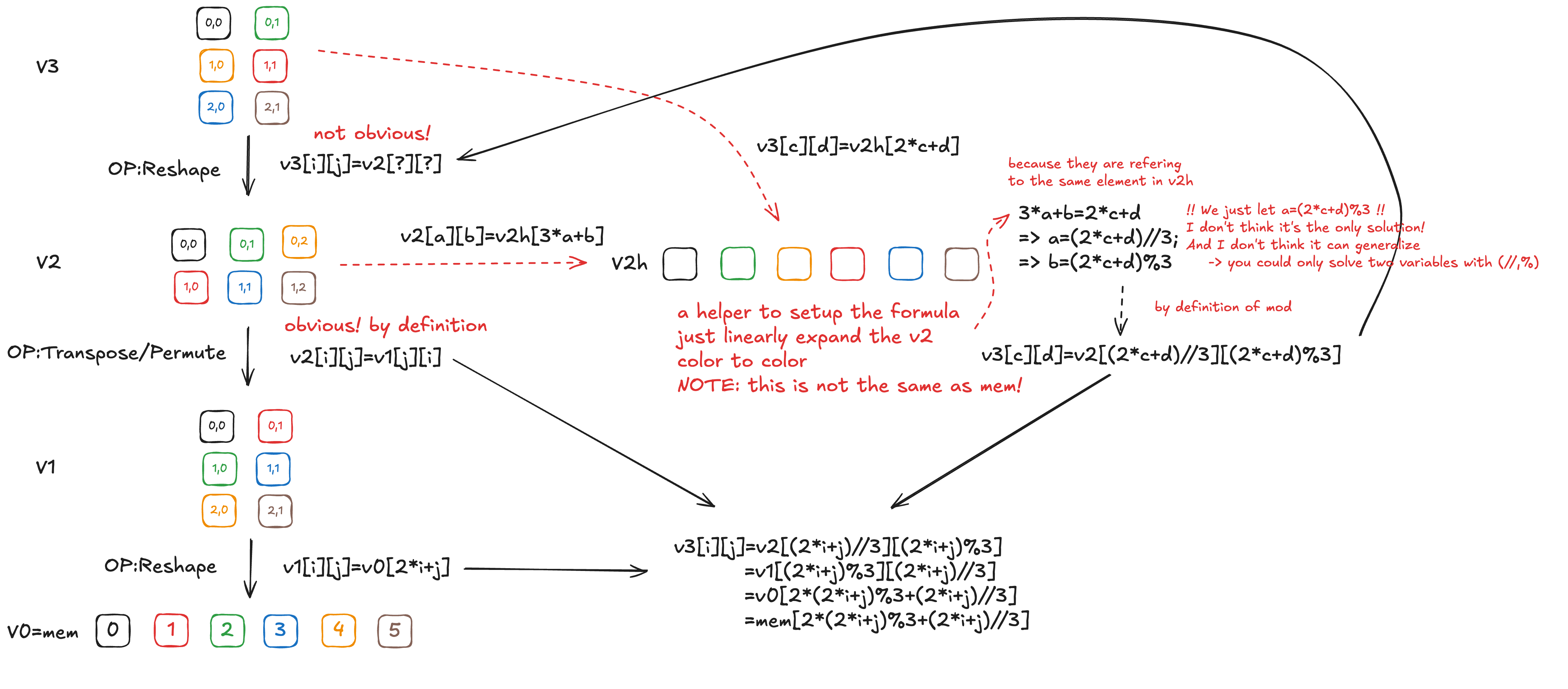
The idea is to render the last view, and project each element onto the first one (the idea also apply if you have more than two views).
First, let’s render the last view, and write down the index for each element, totaling 6 elements
row * 2 + col = index
0   * 2 + 0   = 0x0
0   * 2 + 1   = 0x1
1   * 2 + 0   = 0x2
1   * 2 + 1   = 0x3
2   * 2 + 0   = 0x4
2   * 2 + 1   = 0x5
However, the memory address (index) isn’t the final result, recall that this multi view represent the following transform,
where the memory for the final three by two matrix is 0, 2, 4, 1, 3, 5:
 (3,2)                        (2,3)                    (3,2)
0x00 0x01   transpose    0x00 0x02 0x04  reshape     0x00 0x02
0x02 0x03 ------------>  0x01 0x03 0x05 ---------->  0x04 0x01
0x04 0x05                                            0x03 0x05
So we actually want to project these six address such that their final value look like:
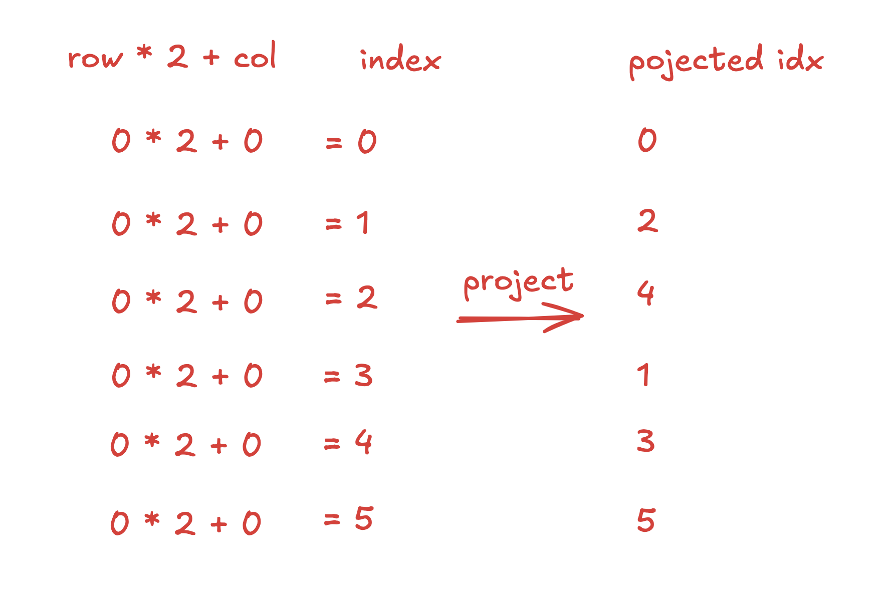
Look at this relation and the rendered expression (I replaced “ridx” with “row” and “col” for readability):
(((((row*2)+col)%3)*2)+(((row*2)+col)//3))

Can you spot the pattern?
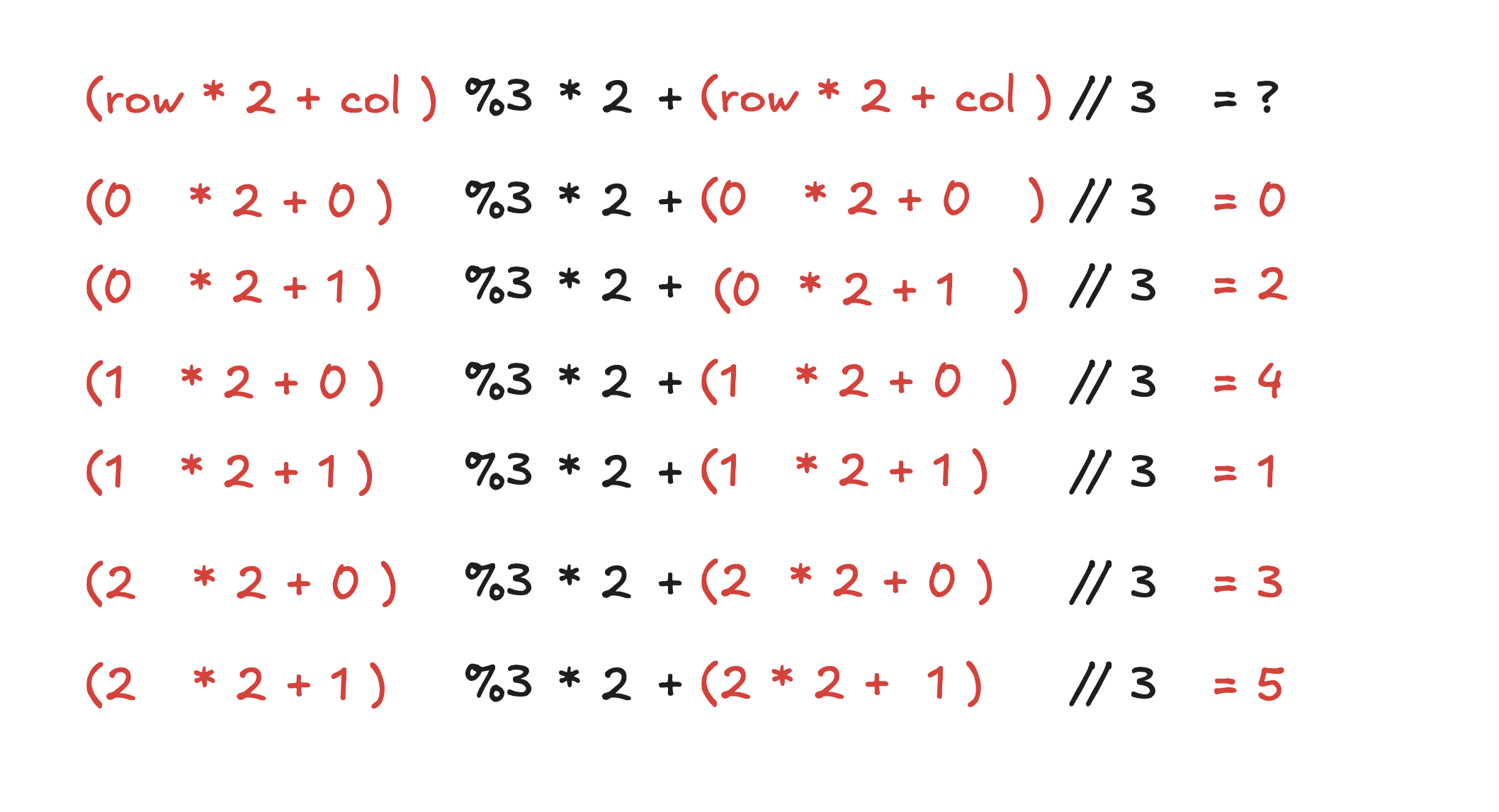
Now, take a guess on what the number 3 and 2 in %3, *2, and //3 each represent:

Note that the two accs are of different values, the one on the left has value 1, the one on the right has value 3, as
you see below, it is accumulating.
Does it look somewhat analogous to this line of code:
    acc, idxs = 1, []
    for d in reversed(view.shape):
      idxs.append((idx//acc)%d)
      acc *= d
In other words, we first render the expression for the last view, the there are two input indices, row and col.
And we get the output expression, row*2+col. The relation between this view, and its previous view, is “(expression // acc) % shape”,
and the “shape” refers to every shape in the previous view. The acc is accumulated as we go through each shape. This
transformed result becomes the input the previous view. The input indices are now (idx // 1) % 3 (row) and (idx // 3) (col),
and we apply the previous’s view’s stride on it, giving us the final result.
You don’t actually need to spot the pattern. Here are some notes to introduce the idea behind this solution:
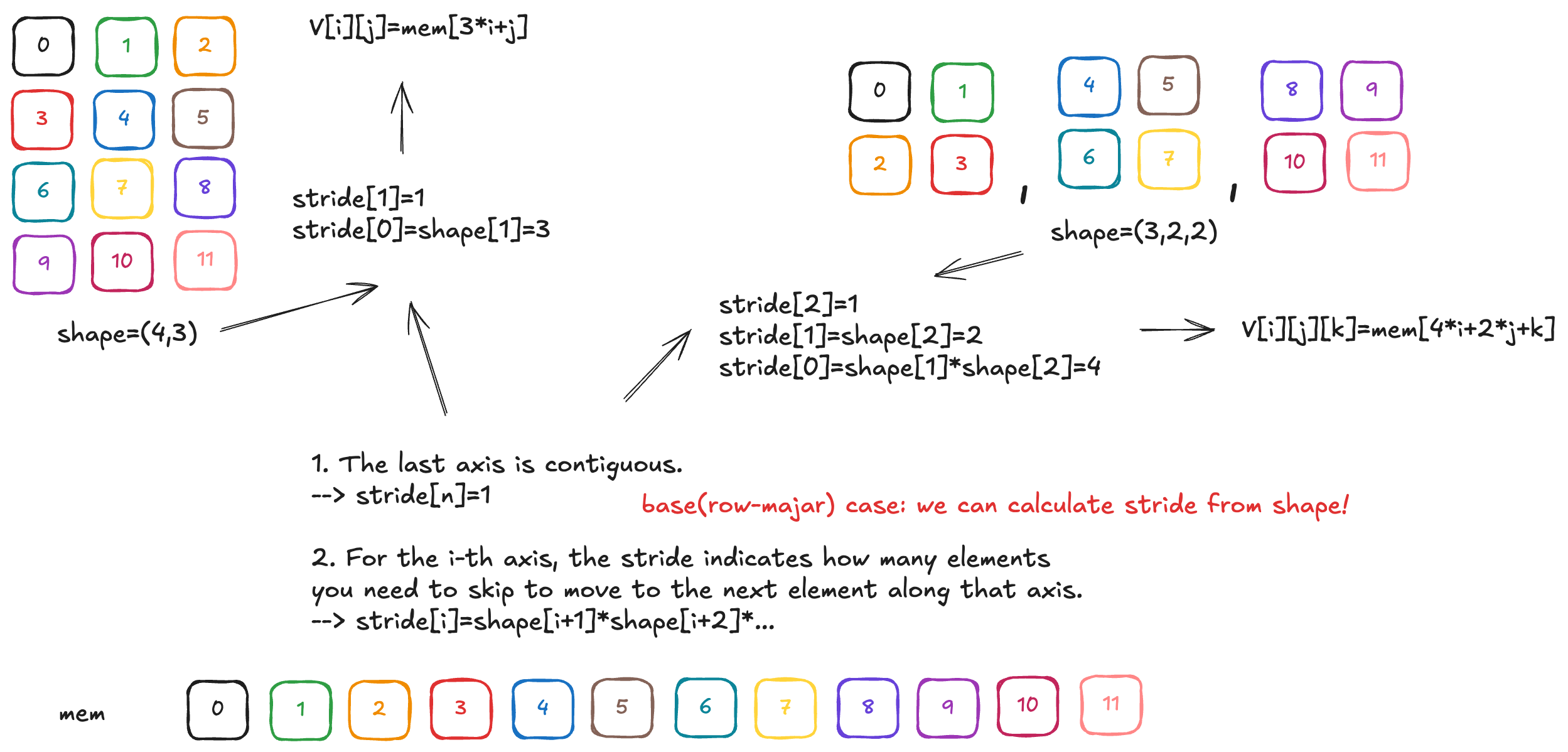
Note: the excali draw file is “img/20250106_st_illustrate.excalidraw”